 |
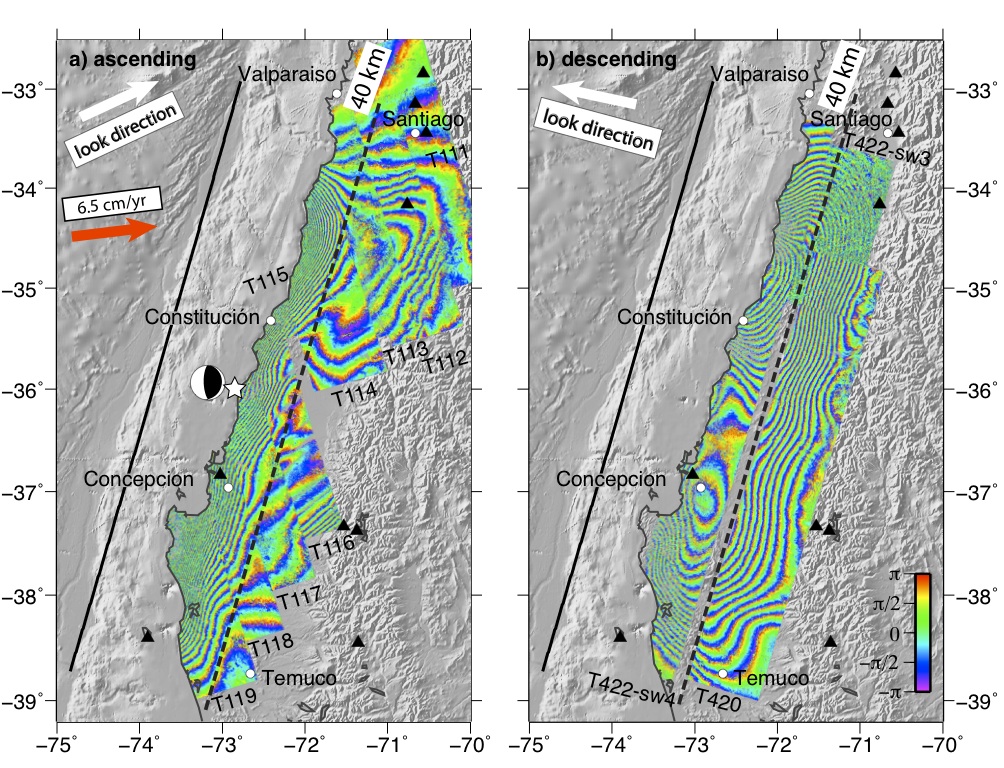
Nine tracks of ALOS ascending interferograms (FBS-FBS mode) and two tracks of ALOS descending interferograms (two subswaths of ScanSAR-ScanSAR mode and ScanSAR-FBS mode, and one track of FBS-FBS mode) cover a wide area from the coastline of central Chile to the foothills of the southern Andes. The white arrows show the radar look direction. The color scale shows the wrapped phase that corresponds to the range change (11.8 cm per cycle) between the ground points and the radar antenna. The ScanSAR acquisition of Track 422 on March 1, 2010 is particularly important for recording the entire coseismic deformation along the coastline of Chile. The white star indicates the earthquake epicenter. The focal mechanism of this earthquake is from Global CMT solution [NEIC, 2010]. The black triangles show the locations of the 13 GPS sites used in the inversion (4 sites are outside of the map boundaries). Solid black line shows the surface trace of the simplified fault model and the dashed black line marks the 40-km depth position of the fault for a 15 degree dip angle. The down-dip slip limit of this earthquake can be infered intuitively by the fringe pattern of the interferograms. Red arrow shows the interseismic convergence vector.
Satellite images were collected by the
L-band synthetic aperture radar
aboard the ALOS spacecraft that is operated by the Japanese Space
Agency - JAXA.
|
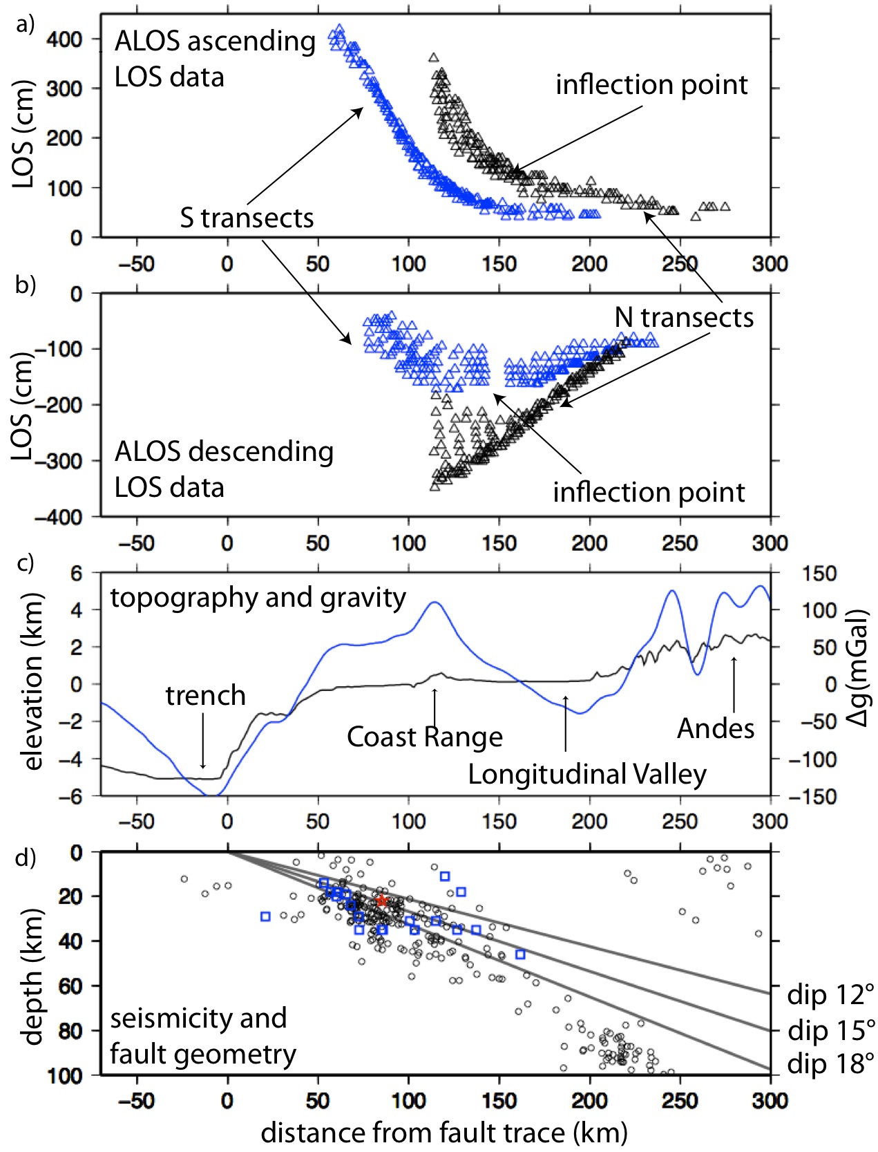
Profiles across the fault
| Transects of unwrapped ALOS line-of-sight data a) ascending and b) descending. Locations of north (black) and south (blue) transects are shown in the figure above. The down-dip slip limit are marked as "inflection point". c) Smoothed topography (black line) and free-air gravity (blue line) profiles over Maule, Chile illustrating major geological features: trench axis, Chilean Coast Range, Longitudinal Valley and High Andes. d) Seismicity and fault geometry in Maule, Chile region. The black circles show the M>4 background seismicity spanning 1960-2007, whose depths are well constrained in EHB bulletin. The red star shows the epicenter of the Maule, Chile earthquake and the blue squares show the locations of the M>6 aftershocks [NEIC, 2010]. Three gray lines show the fault plane for 12°, 15°, 18° dip angles used in the slip models. Note the 12 degree dipping surface lies shallower than the epicenter and much of the background seismicity.
|
 |
Coseismic slip inversion
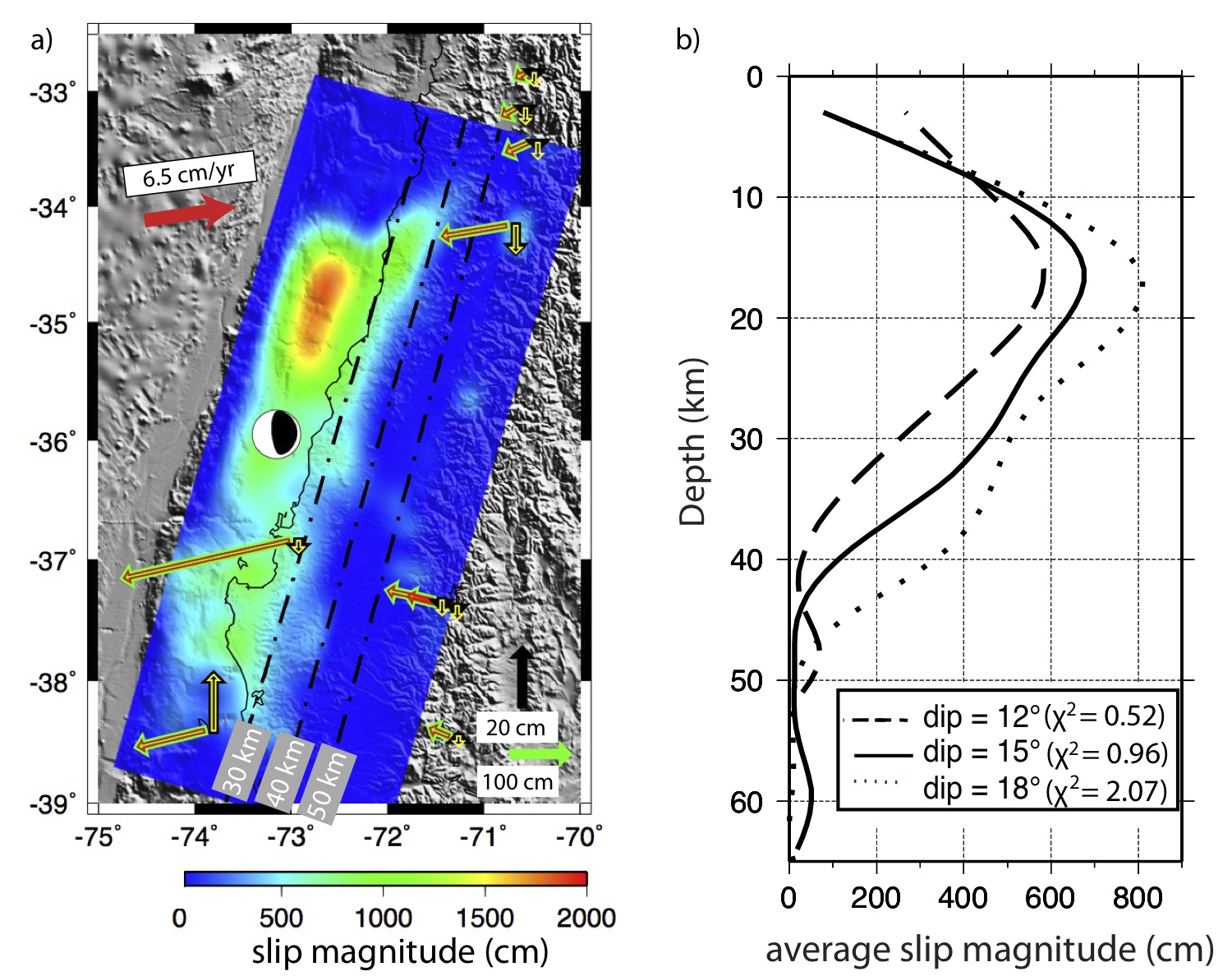 |
Coseismic slip model along a 15° dipping fault plane over shaded topography in Mercator projection. Dashed lines show contours of fault depth (they are not exactly parallel because of the map projection). The red arrows show the observed horizontal displacement of the GPS vectors and the nearly coincident green arrows show the predicted horizontal displacement from the coseismic slip model. Note the directions of coseismic slip from the coastal GPS, and the moment tensor is parallel to the interseismic motion vector indicating a significant right-lateral slip component to accommodate the oblique convergence. b) Along-strike averaged slip versus depth for different dip angles. The solid black line (15° dip) shows the preferred slip-depth distribution. The model misfits for different dip angles are also shown. The possible Moho depth is marked as two gray bars. Note the average slip magnitude decreases more or less linearly from ~18 km depth to ~43 km depth then becomes essentially zero from ~43-48 km depth. The resolution of the inversion under InSAR coverage is about 10 km in absolute depth (40 km along dip) so this slip-depth characteristic is well resolved. The slip offshore is less well constrained.
|
Updated coseismic slip model and static stress change
| We updated the coseismic slip solution with additional published GPS measurements. Then we compared the stress change from this earthquake to the topographic loading stress. See [Luttrell et al., 2011] for details. (a) Coseismic slip model from joint inversion of GPS and InSAR data. The magnitude of slip (hanging wall motion relative to foot wall) are indicated by the colored squares. The dashed gray line indicates the Moho at 40 km depth. (b) and (c) Static shear stress change from Maule, Chile earthquake derived from slip model shown in Figure (a). Positive (negative) shear stress values correspond to stress release (build up). | 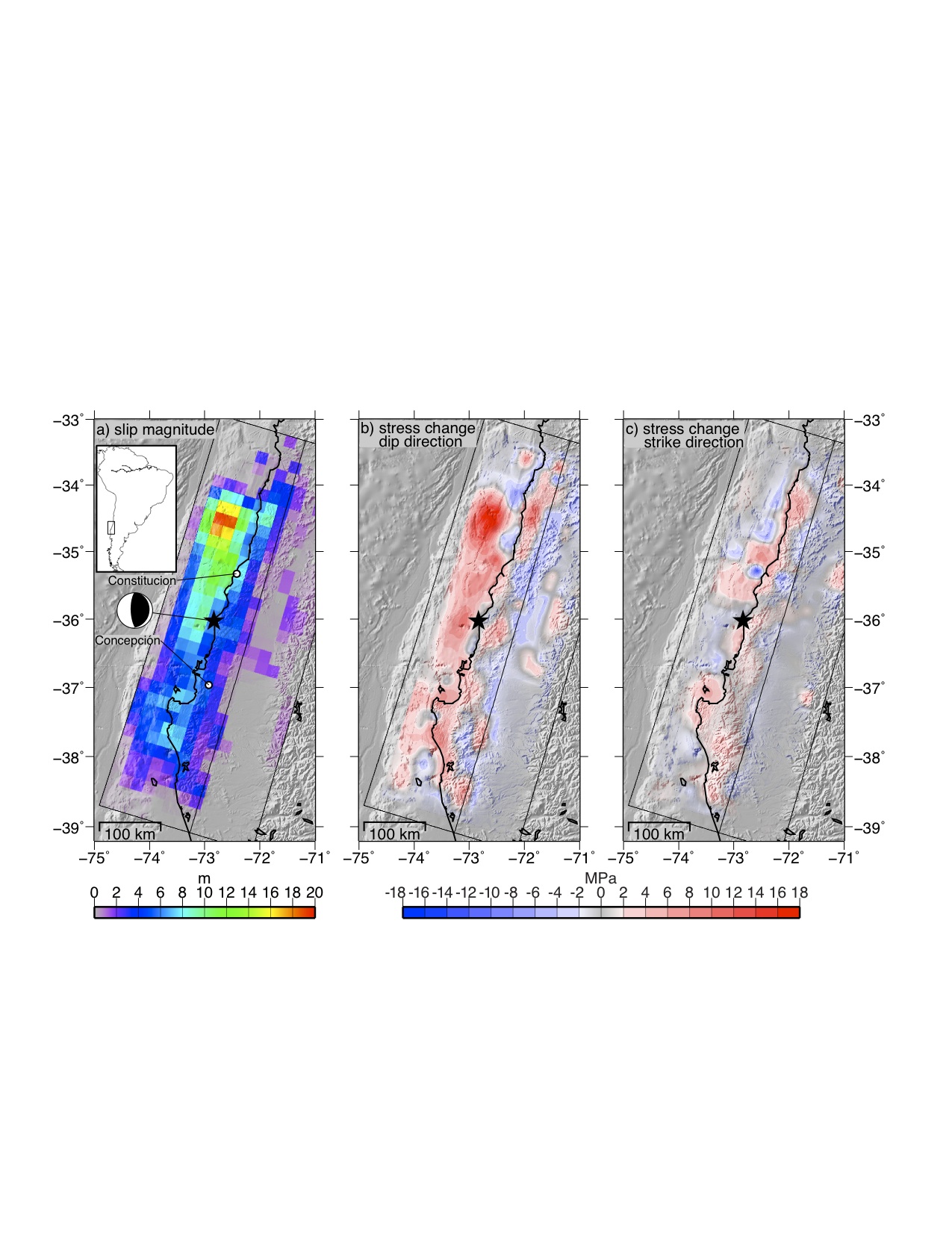 |