Analytic 3-D Elastic Body Force
Model
Smith and Sandwell
[2003]
We
wish to calculate the displacement vector u(x,y,z) on the surface of the Earth due to a
vector body force at depth. This
approach is used to describe motion on both curved and discontinuous faults,
and is also used to evaluate stress regimes above the upper locking depth. For simplicity, we ignore the effects
of Earth’s sphericity. We assume a
Poisson material, and maintain constant moduli with depth. A major difference between this
solution and the Okada
[1985, 1992] solutions
is that we consider deformation due to a vector body force, while the Okada
solution considers deformation due to a dislocation. While the following text provides a brief outline of our
model formulation, the full derivation and source code of our semi-analytic
Fourier model can be found at http://topex.ucsd.edu/body_force/elastic. Our solution is obtained as follows:
(1)
(1)
Develop
three differential equations relating a three-dimensional (3-D) vector body
force to a 3-D vector displacement.
We apply a simple force balance in a homogeneous, isotropic medium and
after a series of substitutions for stress, strain, and displacement, we arrive
at equation A1, where u,v, and
w are vector
displacement components in x, y,
and z,
![]() and
and ![]() are Lame
parameters,
are Lame
parameters, ![]() are vector body
force components:
are vector body
force components:
(2)
A vector
body force is applied at
![]() . To partially
satisfy the boundary condition of zero shear traction at the surface, an image
source is also applied at
. To partially
satisfy the boundary condition of zero shear traction at the surface, an image
source is also applied at ![]() [Weertman, 1964].
Equation A2 describes a point body force at both source and image
locations, where F is
a vector force with units of force.
[Weertman, 1964].
Equation A2 describes a point body force at both source and image
locations, where F is
a vector force with units of force.
![]()
(2)
Take the
3-D Fourier transform of equations A1 and A2 to reduce the partial differential
equations to a set of linear algebraic equations.
(3)
(3)
Invert the linear
system of equations to isolate the 3-D displacement vector solution for U(k), V(k), and W(k).
![]()
![]()
(4)
Perform the
inverse Fourier transform in the z-direction
(depth) by repeated application of the Cauchy Residue Theorem. We assume z to be positive upward.
(5)
Solve the
Boussinesq problem to correct for non-zero normal traction on the
half-space. This derivation
follows the approach of Steketee [1958]
where we impose a negative surface traction in an elastic half space in order
to cancel the non-zero traction from the source and image in the elastic
full-space.
(6)
Integrate
the point source Green's function to simulate a fault. For a complex dipping fault, this integration
could be done numerically.
However, if the faults are assumed to be vertical, the integration can
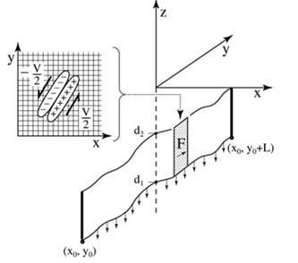
be performed analytically. The
body force is applied between the lower depth d1 (e.g., minus infinity) and the upper
depth d2 (Figure A1). The displacement or stress
(derivatives are computed analytically) can be evaluated at any depth z above d2.
Note that the full displacement solution is the sum of three terms: a
source, an image, and a Boussinesq correction.
(4)

The individual elements of the source and
image tensors are
(5)
![]()
The
individual elements of the Boussinesq correction are
(6)
where
(7)
Construct a
force couple by taking the derivative of the point source in the direction
normal to the fault trace. In
practice, the body forces due to the stress discontinuity across a fault plane
are approximated by the derivative of a Gaussian function, effectively
producing a model fault with a finite thickness (Figure A1). Curved faults are constructed with
overlapping line segments having cosine tapered ends and are typically 6-10 km
long.
The fault trace is imbedded in a
two-dimensional grid which is Fourier transformed, multiplied by the transfer
functions above (5-7), and inverse Fourier transformed. A constant shear
modulus (4.12 x 10¹⁰ Pa) and Poisson ratio (0.25) were adopted for
all calculations. When the lower
edge of the fault is extended to infinite depth, as in the case of the SAF
system model, a Fourier cosine transform
(mirrored pair) is used in the across-fault direction to maintain the
far-field velocity V
step across the plate boundary, effectively conserving moment within the
grid. Note that this requires the
velocity-difference (i.e., stress drop) across a system of connecting faults to
have a constant value ![]() . To avoid
Fourier artifacts where the fault enters the bottom of the grid and leaves the
top of the grid, the fault is extended beyond the top of the model and angled
to match the intersection point at the bottom. (Figure 1) In addition to computing the
velocity field, strain and stress rates are computed from the derivatives of
the model. Horizontal derivatives
are computed by multiplication of
. To avoid
Fourier artifacts where the fault enters the bottom of the grid and leaves the
top of the grid, the fault is extended beyond the top of the model and angled
to match the intersection point at the bottom. (Figure 1) In addition to computing the
velocity field, strain and stress rates are computed from the derivatives of
the model. Horizontal derivatives
are computed by multiplication of ![]() in the Fourier
transform domain and vertical derivatives are computed analytically from the
transfer functions in A5 and A6.
in the Fourier
transform domain and vertical derivatives are computed analytically from the
transfer functions in A5 and A6.
Equations (4-7) were checked using the
computer algebra capabilities in Matlab and then compared to the simple arctangent
function for a two-dimensional fault [Weertman, 1964]
![]() .
.
Of
course, in the two-dimensional case, the Boussinesq correction is not needed
and equation (A-5) reduces to the above arctangent formula. Figure 2 provides a numerical comparison
between the above arctangent function (analytic profile) and our semi-analytic
Fourier solution (Fourier profile). The numerical solutions have relative
errors less than 1% as long as the observation depth z is more than one grid cell size above
the locking depth d2.
The numerical approach is very efficient;
for example, writing and displaying of the deformation/stress grids requires
more computer time than the actual computation of the model. The horizontal
complexity of the fault system has no effect on the speed of the
computation. However, variations
in locking depth along the fault system require computing the model for each
different locking depth and summing the outputs to form the full solution. The
extension to a viscoelastic half space would not introduce a computational
burden on an ordinary workstation.