ES 10 - Homework 3
Plate Tectonics
Greg Anderson and Dave Sandwell

Due 30 January 1998

This homework set is worth a total of 100 points. You will need Handout 2 for problem 4. Please write your answers on paper other than this assignment (except for problems 4 and 5a), make sure your name is on each page, and staple your pages together.

Problem 5 is hard. We encourage you to read the homework before the discussion section on January 26, come to the discussion section that day, and ask questions.

If you have problems or questions, please come to the discussion section, or see me after class, or send me an e-mail. My e-mail address is anderson@python.ucsd.edu.

Problems 1-3: Plate Tectonics (short answer)

Give a sufficiently detailed answer that we know you know what the answer is, but please be concise. Answer in your own words - if you merely copy from the book or lecture notes, you won't get credit. Please note that you will not find the answers to some of these problems in your textbook. You will have to go to other resources (the class web page, the library, etc.) to find those answers.

1. Describe at least five types of evidence which support the plate tectonic model.
2. What are the primary sources of energy for the driving force behind plate tectonics?
3. What is currently believed to be the primary driving force for plate tectonics? What are the other two candidate driving forces?

Problem 4: Plate Motions on a Flat Surface

In this problem, you are going to draw arrows to represent relative plate motion across transform faults, spreading centers, and subduction zones. You will need to look at Handout 2 in order to understand the symbols we use; that handout also has a few examples to try to help clarify things.

Figure 1 shows three plate models on a flat earth. We have indicated spreading centers, subduction zones, and transform faults just as in the examples in Handout 2. We have also indicated the motion of one of the plates in the heavy arrows.

You are to to indicate all the relevant plate motions we have not indicated. This may mean spreading or subduction zones. It also may mean you must indicate relative motion across transform faults. Indicate plate motions by drawing the appropriate arrows on Figure 1.

Problem 5: Seafloor Magnetic Anomalies

At irregular intervals over time, Earth's magnetic field has flipped in such a way that compasses would point south instead of north (as they do now). These flips are called reversals, and they happen for reasons which are not yet understood. The Blue Planet discusses these reversals on pages 137-142.

When new rock is being formed at the mid-ocean ridges, it erupts at a very high temperature (more than 1000° Celsius) and slowly cools. As the rock reaches about 600-700° Celsius, crystals in the rock become oriented in the direction of the magnetic field at the time. This means that rocks which were formed today have crystals aligned with the current ``normal'' polarity of the magnetic field, while rocks which erupted between 0.8 and 1.6 million years ago (Ma) have crystals aligned with the ``reversed'' field which existed at that time.

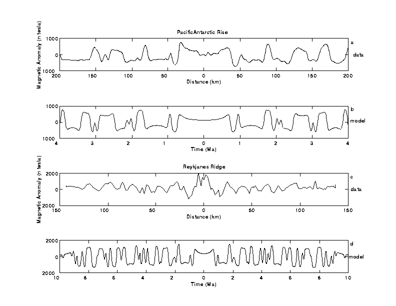
The interaction of the reversing magnetic field and the continuous spreading of the seafloor leaves a magnetic recording on the seafloor. A research vessel crossing perpendicular to a spreading ridge can measure the small variations in magnetic field associated with the rocks on the seafloor, and will see an alternating pattern of magnetic polarities which are called magnetic anomalies. These magnetic anomaly measurements can be used to establish the spreading rate at each ridge.

You will do that in this problem. Figure 2 shows four plots, two for each of two different ridges. Figures 2a and 2b are from the southern East Pacific Rise (latitude 52°S and longitude 118°W) and Figures 2c and 2d are from the Reykjanes Ridge (latitude 61°N and longitude 28°W). Figures 2a and 2c are real data showing magnetic field as a function of distance from the ridge, and Figures 2b and 2d show artificial magnetic fields (created in a computer) as a function of time. From these figures, you will compute spreading rates for each ridge.

Here are the questions you are to answer:

1. Where are these two ridges? Draw an ``X'' at their locations on the world map shown in Figure 3.
2. What two plates are separated by each ridge?
3. Is 1 kilometer/million years equal to 1 millimeter/year? Show your work for full credit.
4. Compare Figures 2a and 2b with each other; you should see that there are peaks and troughs in each profile which seem to match. From left to right, label the most prominent peaks and troughs which correspond to each other A, B, C, etc.
5. Now make a table of time and distance for your labeled peaks.
6. Make a graph of the numbers in this table, with time along the X axis and distance along the Y axis. Using a method similar to that of problem 9 in Homework 1, find the spreading rate in mm/yr for the southern East Pacific Rise.
7. Now repeat parts (d)-(f) with Figures 2c and 2d to find the spreading rate in mm/yr for the Reykjanes Ridge. This will be a bit tough, but then real data is often like that.
8. Turn in your answers to part (a)-(c), your copy of Figure 2 with the peaks labeled as described in part (d), your tables of numbers from part (e), your two graphs from part (f), and your spreading rates in mm/yr.

Figure 1: Plate Diagrams for Problem 4

Figure 2: Magnetic Profiles for Problem 5

Figure 3: World Map for Problem 5

Back to Top
Back to Homework Page
Back to ES 10 Home Page